mmschlk/shapiq
GitHub: mmschlk/shapiq
基于博弈论的机器学习可解释性库,计算任意阶 Shapley 特征交互值以揭示多特征协同效应对模型预测的影响。
Stars: 757 | Forks: 67
# shapiq:用于机器学习的 Shapley 交互  [](https://badge.fury.io/py/shapiq)
[](https://opensource.org/licenses/MIT)
[](https://codecov.io/gh/mmschlk/shapiq)
[](https://github.com/mmschlk/shapiq/blob/main/.github/workflows/ci.yml)
[](https://shapiq.readthedocs.io/en/latest/?badge=latest)
[](https://pypi.org/project/shapiq)
[](https://pypi.org/project/shapiq)
[](https://pepy.tech/project/shapiq)
[](https://github.com/psf/black)
[](https://github.com/mmschlk/shapiq/issues)
[](https://github.com/mmschlk/shapiq/commits/main)
Shapley Interaction Quantification (`shapiq`) 是一个 Python 包,其功能包括:(1)近似计算任意阶的 Shapley 交互,(2)对机器学习的博弈论算法进行基准测试,(3)解释模型预测的特征交互。`shapiq` 对广为人知的 [shap](https://github.com/shap/shap) 包进行了扩展,既适用于研究机器学习中博弈论的科研人员,也适用于需要解释模型的最终用户。SHAP-IQ 通过量化实体(在博弈论术语中称为 **玩家**)之间的 **协同** 效应,扩展了单一的 Shapley value,这些实体可以是解释性特征、数据点或集成模型中的弱学习器。玩家之间的协同效应为机器学习模型提供了更全面的视角。
## 🛠️ 安装
`shapiq` 需要 **Python 3.12 及以上版本**。
可以通过 `uv` 进行安装:
```
uv add shapiq
```
或者通过 `pip`:
```
pip install shapiq
```
## 👀 即将推出
## ⭐ 快速入门
您可以使用 `shapiq.explainer` 解释您的模型,并使用 `shapiq.plot` 可视化 Shapley 交互。
如果您对底层的博弈论算法感兴趣,可以查看 `shapiq.approximator` 和 `shapiq.games` 模块。
### 计算任意阶的特征交互
使用 Shapley 交互解释您的模型:
只需加载您的数据和模型,然后使用 `shapiq.Explainer` 计算 Shapley 交互。
```
import shapiq
# 加载数据
X, y = shapiq.load_california_housing(to_numpy=True)
# 训练模型
from sklearn.ensemble import RandomForestRegressor
model = RandomForestRegressor()
model.fit(X, y)
# 设置 explainer 以获取最高阶数为 4 的 k-SII interaction values
explainer = shapiq.TabularExplainer(
model=model,
data=X,
index="k-SII",
max_order=4
)
# 解释模型对第一个样本的预测
interaction_values = explainer.explain(X[0], budget=256)
# 分析 interaction values
print(interaction_values)
>> InteractionValues(
>> index=k-SII, max_order=4, min_order=0, estimated=False,
>> estimation_budget=256, n_players=8, baseline_value=2.07282292,
>> Top 10 interactions:
>> (0,): 1.696969079 # attribution of feature 0
>> (0, 5): 0.4847876
>> (0, 1): 0.4494288 # interaction between features 0 & 1
>> (0, 6): 0.4477677
>> (1, 5): 0.3750034
>> (4, 5): 0.3468325
>> (0, 3, 6): -0.320 # interaction between features 0 & 3 & 6
>> (2, 3, 6): -0.329
>> (0, 1, 5): -0.363
>> (6,): -0.56358890
>> )
```
### 像使用 SHAP 一样计算 Shapley value
如果您习惯了使用 SHAP,您同样可以按照相同的方式使用 `shapiq` 计算 Shapley value:
您可以加载数据和模型,然后使用 `shapiq.Explainer` 计算 Shapley value。
如果将 index 设置为 ``'SV'``,您将获得与在 SHAP 中一样的 Shapley value。
```
import shapiq
data, model = ... # get your data and model
explainer = shapiq.Explainer(
model=model,
data=data,
index="SV", # Shapley values
)
shapley_values = explainer.explain(data[0])
shapley_values.plot_force(feature_names=...)
```
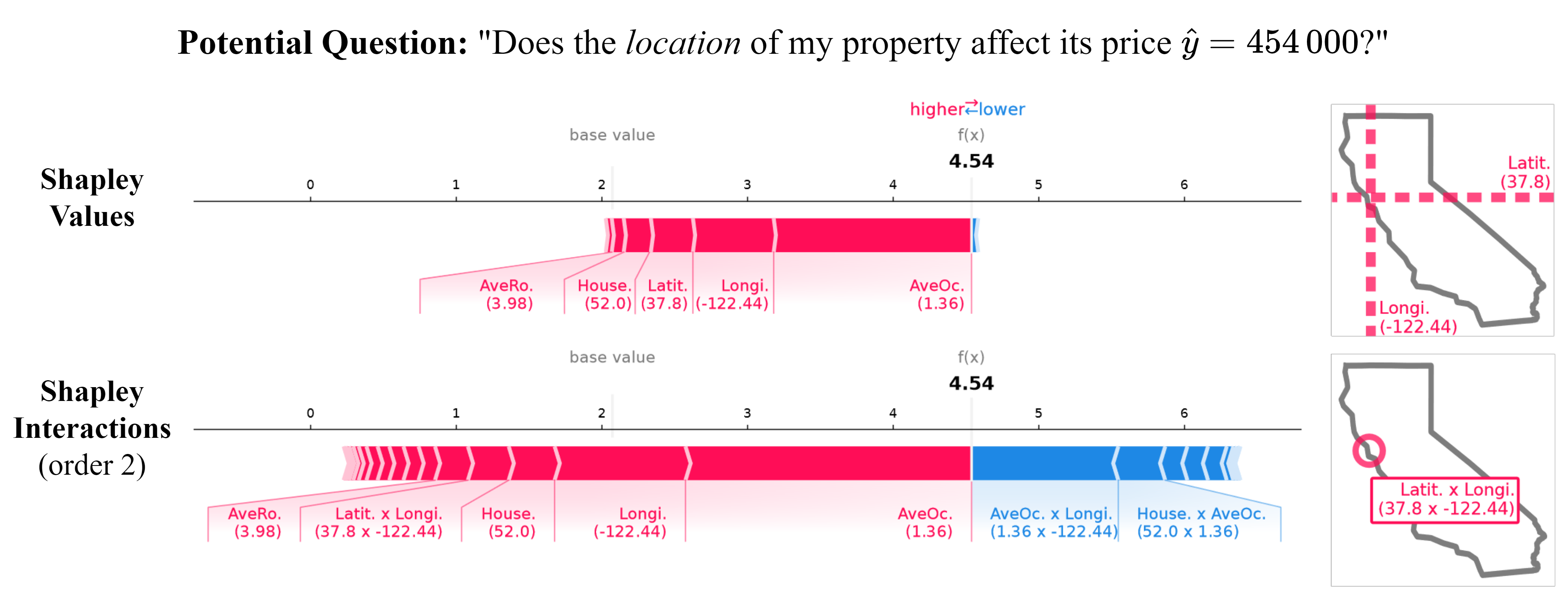
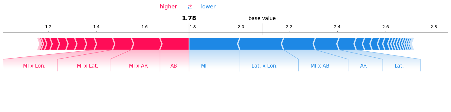
一旦获得了 Shapley value,您也可以轻松计算出交互值:
```
explainer = shapiq.Explainer(
model=model,
data=data,
index="k-SII", # k-SII interaction values
max_order=2 # specify any order you want
)
interaction_values = explainer.explain(data[0])
interaction_values.plot_force(feature_names=...)
```
[](https://badge.fury.io/py/shapiq)
[](https://opensource.org/licenses/MIT)
[](https://codecov.io/gh/mmschlk/shapiq)
[](https://github.com/mmschlk/shapiq/blob/main/.github/workflows/ci.yml)
[](https://shapiq.readthedocs.io/en/latest/?badge=latest)
[](https://pypi.org/project/shapiq)
[](https://pypi.org/project/shapiq)
[](https://pepy.tech/project/shapiq)
[](https://github.com/psf/black)
[](https://github.com/mmschlk/shapiq/issues)
[](https://github.com/mmschlk/shapiq/commits/main)
Shapley Interaction Quantification (`shapiq`) 是一个 Python 包,其功能包括:(1)近似计算任意阶的 Shapley 交互,(2)对机器学习的博弈论算法进行基准测试,(3)解释模型预测的特征交互。`shapiq` 对广为人知的 [shap](https://github.com/shap/shap) 包进行了扩展,既适用于研究机器学习中博弈论的科研人员,也适用于需要解释模型的最终用户。SHAP-IQ 通过量化实体(在博弈论术语中称为 **玩家**)之间的 **协同** 效应,扩展了单一的 Shapley value,这些实体可以是解释性特征、数据点或集成模型中的弱学习器。玩家之间的协同效应为机器学习模型提供了更全面的视角。
## 🛠️ 安装
`shapiq` 需要 **Python 3.12 及以上版本**。
可以通过 `uv` 进行安装:
```
uv add shapiq
```
或者通过 `pip`:
```
pip install shapiq
```
## 👀 即将推出
## ⭐ 快速入门
您可以使用 `shapiq.explainer` 解释您的模型,并使用 `shapiq.plot` 可视化 Shapley 交互。
如果您对底层的博弈论算法感兴趣,可以查看 `shapiq.approximator` 和 `shapiq.games` 模块。
### 计算任意阶的特征交互
使用 Shapley 交互解释您的模型:
只需加载您的数据和模型,然后使用 `shapiq.Explainer` 计算 Shapley 交互。
```
import shapiq
# 加载数据
X, y = shapiq.load_california_housing(to_numpy=True)
# 训练模型
from sklearn.ensemble import RandomForestRegressor
model = RandomForestRegressor()
model.fit(X, y)
# 设置 explainer 以获取最高阶数为 4 的 k-SII interaction values
explainer = shapiq.TabularExplainer(
model=model,
data=X,
index="k-SII",
max_order=4
)
# 解释模型对第一个样本的预测
interaction_values = explainer.explain(X[0], budget=256)
# 分析 interaction values
print(interaction_values)
>> InteractionValues(
>> index=k-SII, max_order=4, min_order=0, estimated=False,
>> estimation_budget=256, n_players=8, baseline_value=2.07282292,
>> Top 10 interactions:
>> (0,): 1.696969079 # attribution of feature 0
>> (0, 5): 0.4847876
>> (0, 1): 0.4494288 # interaction between features 0 & 1
>> (0, 6): 0.4477677
>> (1, 5): 0.3750034
>> (4, 5): 0.3468325
>> (0, 3, 6): -0.320 # interaction between features 0 & 3 & 6
>> (2, 3, 6): -0.329
>> (0, 1, 5): -0.363
>> (6,): -0.56358890
>> )
```
### 像使用 SHAP 一样计算 Shapley value
如果您习惯了使用 SHAP,您同样可以按照相同的方式使用 `shapiq` 计算 Shapley value:
您可以加载数据和模型,然后使用 `shapiq.Explainer` 计算 Shapley value。
如果将 index 设置为 ``'SV'``,您将获得与在 SHAP 中一样的 Shapley value。
```
import shapiq
data, model = ... # get your data and model
explainer = shapiq.Explainer(
model=model,
data=data,
index="SV", # Shapley values
)
shapley_values = explainer.explain(data[0])
shapley_values.plot_force(feature_names=...)
```
一旦获得了 Shapley value,您也可以轻松计算出交互值:
```
explainer = shapiq.Explainer(
model=model,
data=data,
index="k-SII", # k-SII interaction values
max_order=2 # specify any order you want
)
interaction_values = explainer.explain(data[0])
interaction_values.plot_force(feature_names=...)
```
 对于大规模的用例,您还可以查看 [👓``ProxySPEX``](https://shapiq.readthedocs.io/en/latest/api/shapiq.approximator.sparse.html#shapiq.approximator.sparse.SPEX) approxator。
```
# 加载你的大量 features 的数据和模型
data, model, n_features = ...
# 直接使用 ProxySPEX approximator
approximator = shapiq.ProxySPEX(n=n_features, index="FBII", max_order=2)
fbii_scores = approximator.approximate(budget=2000, game=model.predict)
# 或者使用 ProxySPEX 和 explainer
explainer = shapiq.Explainer(
model=model,
data=data,
index="FBII",
max_order=2,
approximator="proxyspex" # specify ProxySPEX as approximator
)
explanation = explainer.explain(data[0])
```
### 可视化特征交互
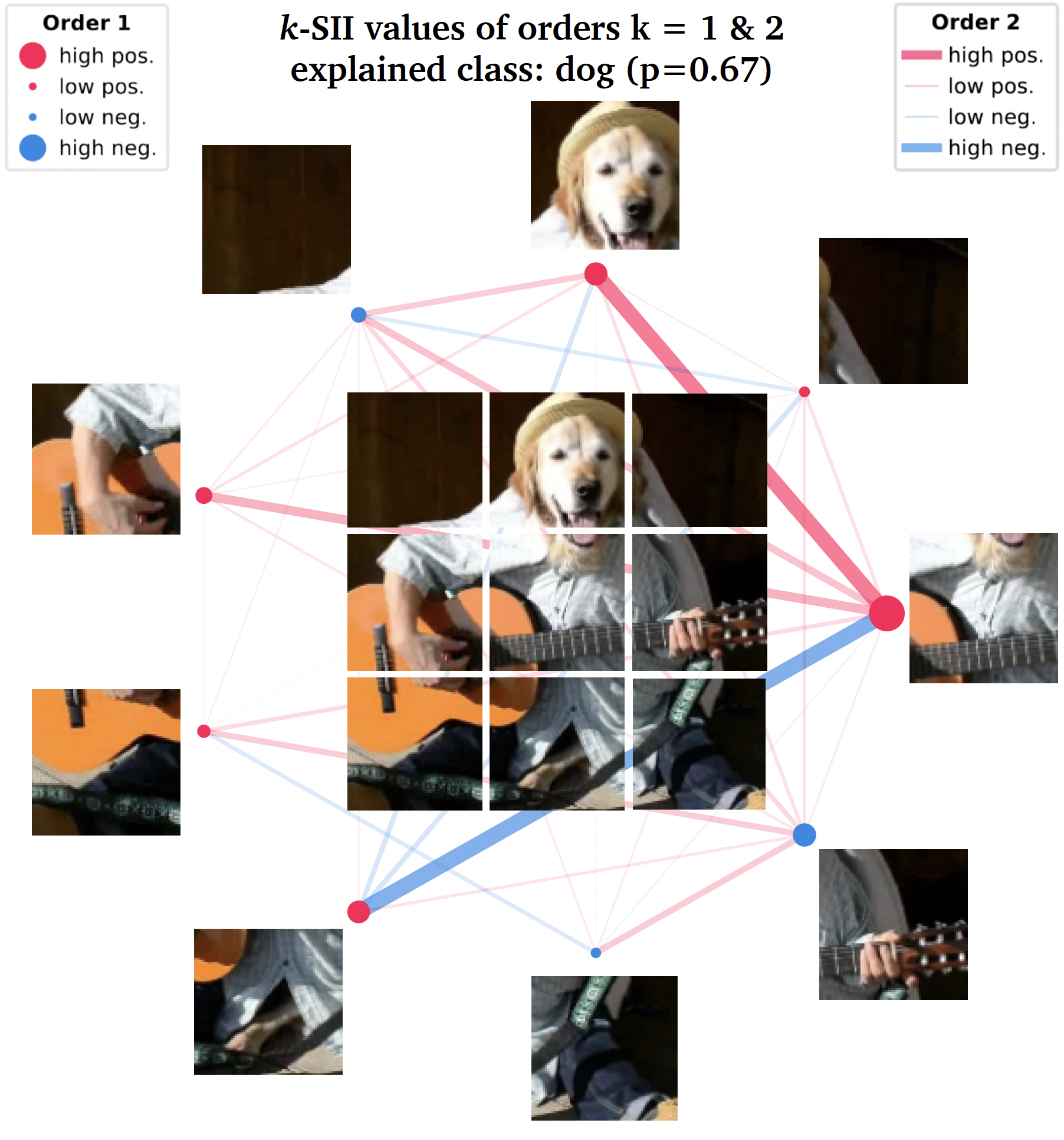
网络图是一种可视化 2 阶及以下交互分数的便捷方式。
您可以在下面看到此类图表的示例。
节点表示特征 **归因**,边表示特征之间的 **交互**。
节点和边的强度与大小分别与归因和交互的绝对值成正比。
```
shapiq.network_plot(
first_order_values=interaction_values.get_n_order_values(1),
second_order_values=interaction_values.get_n_order_values(2)
)
# 或者使用
interaction_values.plot_network()
```
上面的伪代码可以生成以下图表(此处也添加了一张图片):
对于大规模的用例,您还可以查看 [👓``ProxySPEX``](https://shapiq.readthedocs.io/en/latest/api/shapiq.approximator.sparse.html#shapiq.approximator.sparse.SPEX) approxator。
```
# 加载你的大量 features 的数据和模型
data, model, n_features = ...
# 直接使用 ProxySPEX approximator
approximator = shapiq.ProxySPEX(n=n_features, index="FBII", max_order=2)
fbii_scores = approximator.approximate(budget=2000, game=model.predict)
# 或者使用 ProxySPEX 和 explainer
explainer = shapiq.Explainer(
model=model,
data=data,
index="FBII",
max_order=2,
approximator="proxyspex" # specify ProxySPEX as approximator
)
explanation = explainer.explain(data[0])
```
### 可视化特征交互
网络图是一种可视化 2 阶及以下交互分数的便捷方式。
您可以在下面看到此类图表的示例。
节点表示特征 **归因**,边表示特征之间的 **交互**。
节点和边的强度与大小分别与归因和交互的绝对值成正比。
```
shapiq.network_plot(
first_order_values=interaction_values.get_n_order_values(1),
second_order_values=interaction_values.get_n_order_values(2)
)
# 或者使用
interaction_values.plot_network()
```
上面的伪代码可以生成以下图表(此处也添加了一张图片):
[](https://badge.fury.io/py/shapiq)
[](https://opensource.org/licenses/MIT)
[](https://codecov.io/gh/mmschlk/shapiq)
[](https://github.com/mmschlk/shapiq/blob/main/.github/workflows/ci.yml)
[](https://shapiq.readthedocs.io/en/latest/?badge=latest)
[](https://pypi.org/project/shapiq)
[](https://pypi.org/project/shapiq)
[](https://pepy.tech/project/shapiq)
[](https://github.com/psf/black)
[](https://github.com/mmschlk/shapiq/issues)
[](https://github.com/mmschlk/shapiq/commits/main)
Shapley Interaction Quantification (`shapiq`) 是一个 Python 包,其功能包括:(1)近似计算任意阶的 Shapley 交互,(2)对机器学习的博弈论算法进行基准测试,(3)解释模型预测的特征交互。`shapiq` 对广为人知的 [shap](https://github.com/shap/shap) 包进行了扩展,既适用于研究机器学习中博弈论的科研人员,也适用于需要解释模型的最终用户。SHAP-IQ 通过量化实体(在博弈论术语中称为 **玩家**)之间的 **协同** 效应,扩展了单一的 Shapley value,这些实体可以是解释性特征、数据点或集成模型中的弱学习器。玩家之间的协同效应为机器学习模型提供了更全面的视角。
## 🛠️ 安装
`shapiq` 需要 **Python 3.12 及以上版本**。
可以通过 `uv` 进行安装:
```
uv add shapiq
```
或者通过 `pip`:
```
pip install shapiq
```
## 👀 即将推出
## ⭐ 快速入门
您可以使用 `shapiq.explainer` 解释您的模型,并使用 `shapiq.plot` 可视化 Shapley 交互。
如果您对底层的博弈论算法感兴趣,可以查看 `shapiq.approximator` 和 `shapiq.games` 模块。
### 计算任意阶的特征交互
使用 Shapley 交互解释您的模型:
只需加载您的数据和模型,然后使用 `shapiq.Explainer` 计算 Shapley 交互。
```
import shapiq
# 加载数据
X, y = shapiq.load_california_housing(to_numpy=True)
# 训练模型
from sklearn.ensemble import RandomForestRegressor
model = RandomForestRegressor()
model.fit(X, y)
# 设置 explainer 以获取最高阶数为 4 的 k-SII interaction values
explainer = shapiq.TabularExplainer(
model=model,
data=X,
index="k-SII",
max_order=4
)
# 解释模型对第一个样本的预测
interaction_values = explainer.explain(X[0], budget=256)
# 分析 interaction values
print(interaction_values)
>> InteractionValues(
>> index=k-SII, max_order=4, min_order=0, estimated=False,
>> estimation_budget=256, n_players=8, baseline_value=2.07282292,
>> Top 10 interactions:
>> (0,): 1.696969079 # attribution of feature 0
>> (0, 5): 0.4847876
>> (0, 1): 0.4494288 # interaction between features 0 & 1
>> (0, 6): 0.4477677
>> (1, 5): 0.3750034
>> (4, 5): 0.3468325
>> (0, 3, 6): -0.320 # interaction between features 0 & 3 & 6
>> (2, 3, 6): -0.329
>> (0, 1, 5): -0.363
>> (6,): -0.56358890
>> )
```
### 像使用 SHAP 一样计算 Shapley value
如果您习惯了使用 SHAP,您同样可以按照相同的方式使用 `shapiq` 计算 Shapley value:
您可以加载数据和模型,然后使用 `shapiq.Explainer` 计算 Shapley value。
如果将 index 设置为 ``'SV'``,您将获得与在 SHAP 中一样的 Shapley value。
```
import shapiq
data, model = ... # get your data and model
explainer = shapiq.Explainer(
model=model,
data=data,
index="SV", # Shapley values
)
shapley_values = explainer.explain(data[0])
shapley_values.plot_force(feature_names=...)
```
一旦获得了 Shapley value,您也可以轻松计算出交互值:
```
explainer = shapiq.Explainer(
model=model,
data=data,
index="k-SII", # k-SII interaction values
max_order=2 # specify any order you want
)
interaction_values = explainer.explain(data[0])
interaction_values.plot_force(feature_names=...)
```
对于大规模的用例,您还可以查看 [👓``ProxySPEX``](https://shapiq.readthedocs.io/en/latest/api/shapiq.approximator.sparse.html#shapiq.approximator.sparse.SPEX) approxator。
```
# 加载你的大量 features 的数据和模型
data, model, n_features = ...
# 直接使用 ProxySPEX approximator
approximator = shapiq.ProxySPEX(n=n_features, index="FBII", max_order=2)
fbii_scores = approximator.approximate(budget=2000, game=model.predict)
# 或者使用 ProxySPEX 和 explainer
explainer = shapiq.Explainer(
model=model,
data=data,
index="FBII",
max_order=2,
approximator="proxyspex" # specify ProxySPEX as approximator
)
explanation = explainer.explain(data[0])
```
### 可视化特征交互
网络图是一种可视化 2 阶及以下交互分数的便捷方式。
您可以在下面看到此类图表的示例。
节点表示特征 **归因**,边表示特征之间的 **交互**。
节点和边的强度与大小分别与归因和交互的绝对值成正比。
```
shapiq.network_plot(
first_order_values=interaction_values.get_n_order_values(1),
second_order_values=interaction_values.get_n_order_values(2)
)
# 或者使用
interaction_values.plot_network()
```
上面的伪代码可以生成以下图表(此处也添加了一张图片):
标签:逆向工具