pyTECTOR 是 Angelier 古應力反演程式 TENSOR 5.45 的 Python 重建版,依論文重寫演算法並逐位驗證,同時新增回轉、tilt test 與逐筆影響力診斷等功能。
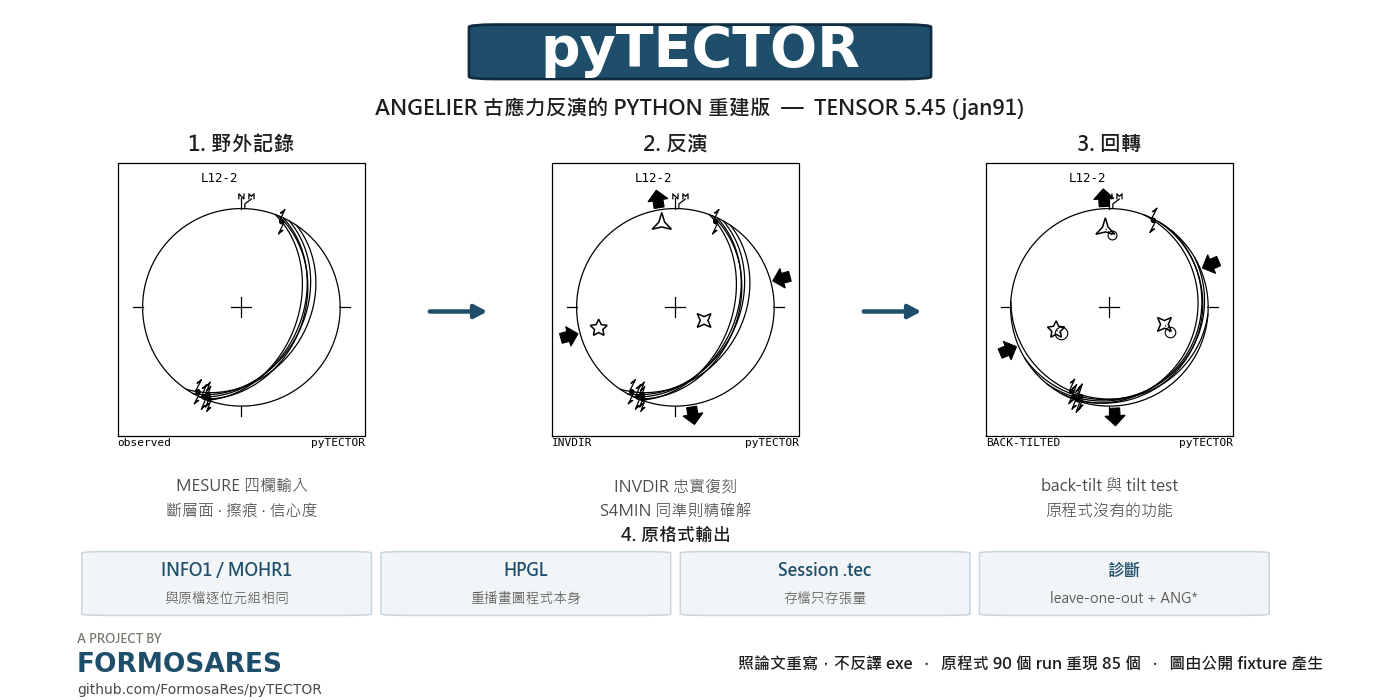
**Angelier 古應力反演的 Python 重建版,對應 TENSOR 5.45 (jan91)**
照論文重寫,不反譯執行檔;原程式 90 個 run 重現 85 個;回轉與 tilt test;逐筆影響力診斷;INFO1/MOHR1/HPGL 原格式輸出
[](docs/mesure_oracle.md)
[](pyproject.toml)
[](#quick-start)
[](tests/)
[](tests/test_replication.py)
[](LICENSE)
[使用手冊 中文](docs/manual.zh.md) · [English manual](docs/manual.en.md) · [原程式對話全文](docs/mesure_oracle.md) · [English below](#english)
Angelier 的直接反演法從一組斷層面與擦痕線理,解出最能解釋它們的簡化應力張量,
也就是三個主應力方向與形狀比 Φ。`Tensor.exe` 自 1991 年起執行這項計算,
大量已發表的古應力研究皆建立在其結果之上。
pyTECTOR 執行相同的運算、讀寫相同的檔案、繪製相同的圖,並補上原程式沒有的部分:
**回轉(back-tilt)**、**tilt test**,以及**把同一個準則真正最小化**的第二種跑法,
用來分辨一個答案有多少來自方法本身、多少來自資料。
名稱取自 **TECTOR**,即 Angelier 為這套程式的構造方位資料庫所取的名稱,
印在它產生的每一份 INFO1 上。
## 📸 長什麼樣
| 兩種跑法並列 | 回轉與 tilt test |
|---|---|
|  |  |
## ✨ 核心特色
- **照論文重寫,不反譯執行檔。** 演算法在 Angelier (1984, 1990) 已完整發表,
依論文重建比逆向那個 16 位元二進位快上一個量級。
- **對原程式逐位驗證。** 以 archive 中 92 個 run 作為回歸測試集:前向量
(SIGMN/TAU/TAUST/RUP/ANG)逐筆吻合至檔案精度;以各站記錄的 pass 數與
LAMBDA 重跑後,**85/90 站三軸角度差小於 3°**。
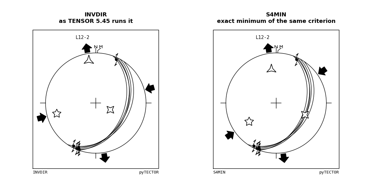
- **INVDIR/S4MIN 兩種跑法並列。** 前者是 Angelier 原方法、原程式的跑法,
後者是同一準則的精確最小值。兩者皆非「真應力」:υ 準則本身有系統性偏差,
即使餵入零雜訊的理想合成資料,仍與真實張量相差約 4°。並列是為了呈現差異
所在,而非在其中擇一。
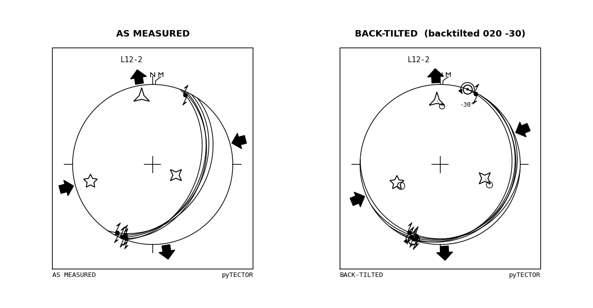
- **回轉與 tilt test,原程式沒有的功能。** 角度以拉桿試誤調整,σ₁σ₂σ₃ 即時重算。
對 INVDIR 而言,回轉前後軸的差距反映的是方法本身的性質而非地質意義
(14 組 archive 配對,實測中位數 σ₁ 差 10.4°)。
- **逐筆影響力診斷。** 「擬合誤差大」與「決定了答案」是兩件不同的事。程式做
leave-one-out 重新反演,並提供**剔除後殘差** ANG\*/RUP\*,同時把「全部資料」
與「剔除後」兩個答案並列寫進匯出的 INFO1。
- **原格式輸出。** INFO1/MOHR1 與原始檔案逐位元組相同;HPGL 匯出是重播原本的
繪圖程式本身,而非另一套獨立實作。
- **Session 存檔。** 全部工作狀態存成單一 JSON;只保存張量,其餘數值於載入時
重新計算,因此存檔中的 Φ 不可能與存檔中的張量互相矛盾。
# English
## What this is
Angelier's direct inversion method takes a set of measured fault planes and
slickenside lineations and returns the reduced stress tensor that best explains
them: the three principal stress directions and the shape ratio Φ. His program
`Tensor.exe` did this from 1991 onwards and a great deal of published
palaeostress work rests on it.
pyTECTOR performs the same arithmetic, reads and writes the same files, draws the
same diagrams, and adds the parts the original never had: back-tilting, a tilt
test, and a second run that minimises the same criterion properly, so that how
much of an answer comes from the method rather than the data can be assessed.
## Provenance
The algorithm is fully published, so this was rebuilt from the papers rather
than by decompiling the 16-bit original: compilation had discarded the names,
the types and the structure, and segmented addressing makes pointers
unresolvable. The work went into reading Angelier (1984, 1990, 1994) and into
measuring the original's own output for everything the papers do not state.
The name is Angelier's too. His papers never name a program, but the binary
names itself in every INFO1 it wrote, and one of the two names on that banner
is **TECTOR**, its tectonic-orientation data base. "TENSOR" was unavailable:
in this field it now means Delvaux's unrelated Win-Tensor, and on PyPI
`pytensor` is PyMC's array library.
Both questions in full, with the banner text and the references:
**[docs/background.en.md](docs/background.en.md)**.
## Quick start
One-click on Windows: download the repository, double-click **`install.bat`**.
It finds a Python (Anaconda first), installs numpy, scipy, matplotlib and
PyQt5, and puts a pyTECTOR shortcut on the desktop. Alternatively
`pip install .` (or `pip install git+https://github.com/FormosaRes/pyTECTOR`)
installs a `pytector` command.
pyTECTOR.bat desktop interface (Windows)
./pyTECTOR.command desktop interface (macOS, Linux)
python demo_report.py [site file] invert an old site, print INFO1 + MOHR1
python run_batch.py [root] [out.csv] both runs over a whole folder tree
**macOS and Linux.** Nothing in the library is Windows-specific, so the
inversion, the file readers and the exports all run unchanged. Install the four
dependencies and use `pyTECTOR.command`, which is double-clickable in Finder:
python3 -m pip install numpy scipy matplotlib PyQt5
./pyTECTOR.command
Two things to know. On an **Apple Silicon** Mac, PyQt5 needs a release with an
arm64 wheel (5.15.10 or newer); if pip starts compiling Qt from source, install
it through conda instead (`conda install -c conda-forge pyqt`). And set
`PYTECTOR_PYTHON` if the launcher should use a particular interpreter rather
than the first one on `PATH` that can import PyQt5. The interface has not been
tested on macOS: the font stacks name macOS and Linux faces so the fixed-width
tables stay aligned, but reports of anything that looks wrong are welcome.
The full interface walkthrough, control by control, is in
**[docs/manual.en.md](docs/manual.en.md)**.
Type a fault in four fields and watch it land on the stereogram:
CS - 122 - 87W - 124
| | | |
| | | +-- pitch and quadrant (62N), or a bare trend (124)
| | +-------- dip and its quadrant
| +-------------- strike
+------------------- confidence C/P/S + movement I/N/S/D
Or open an old run directly: point it at the extension-less data file named
after the site, for example `L12`, and everything loads, INFO1 and all.
## The criterion
| | |
|---|---|
| stress vector | σ = **T**·n (eq 3) |
| shear traction | τ = σ − (n·σ)n (eq 4-5) |
| upsilon vector | λs = τ + υ (eq 12) |
| **objective** | **υ² = λ² + \|τ\|² − 2λ(s·σ)** (eq A1), minimise **S₄ = Συ²** (eq 13) |
| quality | RUP = 100·\|υ\|/(√3/2), 0-200 % ; ANG = angle(s, τ), 0-180° |
The reduced stress tensor is normalised so that the **sum of squared
eigenvalues is 3/2** (eq A16), not so that σ₁ − σ₃ is fixed. The two agree only
at Φ = 0.5, and the criterion is not scale invariant, so this matters.
**The criterion is biased, and that is not a bug in anyone's code.** υ asks for
two things at once: that the predicted shear points along the observed slip,
and that its magnitude is close to λ. Fed perfect Bott data with no noise at
all, it still misses the true tensor by about 4 degrees, because it favours
orientations that put high shear on the faults. The angle-only criterion F2
recovers the same data to 0.00 degrees. This is the root of why TectonicsFP and
similar programs disagree with Angelier's numbers.
## Two runs: INVDIR and S4MIN
Named after what they are, not by a letter that would imply one is better.
**Neither is "the true stress"**, for the reason above.
### INVDIR
`pytector.invdir`, code `INVD`, as TENSOR 5.45 runs it.
Uses Angelier's own (α, β, γ, ψ) parametrisation, equation (14), printed as
(A2) in the appendix:
T = [[cos ψ, α, γ ],
[α, cos(ψ+2π/3), β ],
[γ, β, cos(ψ+4π/3)]]
This tensor is **not** normalised: its entries square to 3/2 + 2(α²+β²+γ²), so
its maximum shear moves as the solution moves. That is exactly why λ has to be
re-adjusted over successive passes, and why the `LAMBDA` printed in INFO1 comes
out smaller than √3/2. The pipeline is:
1. **INVDIR pass k**: minimise S₄ at the current λ, then set λ to the taumax of
the result. The `(NO k)` printed in INFO1 **is the pass number**, not a
choice between two solutions.
2. **PSIDIR**: freeze the axes, switch to the normalised A16 form, λ = √3/2, and
re-minimise over ψ across a **full turn**. This fixes Φ and repairs the
artificial σ₁/σ₃ permutations the unnormalised pass can produce.
Two points are relevant to any reimplementation. υ² is *quadratic* in (α, β, γ)
at fixed ψ, so the inner minimisation is an exact 3×3 linear solve; Angelier's
Appendix I and II perform that expansion by hand, and the polynomials are
regenerated numerically here because the appendix is illegible in the available
scan. Second, ψ must be scanned over the whole circle: restricting it to
[0, π/3] yields Φ = 0 and the wrong axes, because the minimum often sits near
ψ = 336-353°.
### S4MIN
`pytector.modern`, code `S4MN`, the exact minimum of the same S₄.
Eigen-decomposition parametrisation, so λ is the constant √3/2 by construction
and no adjustment loop is needed; the search is global. It reaches a lower S₄ on
**all 92 archive sites**, without exception:
| site | INVDIR S₄ | S4MIN S₄ |
|---|---|---|
| L12 | 0.3018 | 0.2360 |
| 0406-7 | 7.6198 | 7.3201 |
So the original program does not reach the minimum of its own criterion, because
λ stops before it converges.
### Going further
The two runs, PSIDIR's axis relabelling, what λ actually is, why the iteration
diverges, how to read convergence off an INFO1, and the equivariance data
behind the back-tilt warning above are all set out in
**[docs/method.en.md](docs/method.en.md)**.
File formats, the HPGL drawing reference and the repository layout are in
**[docs/formats.en.md](docs/formats.en.md)**.
## Back-tilting
Back-tilting has a window of its own, opened from the toolbar. The main window
shows the data as measured and nothing else, so a stereogram there never needs a
caption to say which orientation it is in.
The window rotates the data, inverts both states, and shows them side by side:
measured on the left, restored on the right, with the numbers for both
underneath. Three ways to set the rotation:
| mode | input | what it does |
|---|---|---|
| reference surface | strike / dip, or its pole as trend / plunge | the rotation that restores that surface to horizontal |
| rotation axis | trend / plunge / angle | applies it directly, right-hand rule |
| partial | 0 to 125 % | any fraction of either of the above |
Both the fault normals and the slip vectors are rotated, so rakes and senses
carry through. The convention was fixed against the archive rather than assumed:
solving for the rotation between an original site and its back-tilted copy
(Kabsch on the fault normals) reproduces all seven cases to better than 2°.
Reference surfaces are drawn as dashed great circles with their poles, and they
rotate with the data, so a correct restoration is visible: the dashed circle
flattens onto the primitive and the pole walks in to the centre.
**The angle is not computed.** There is no analytical solution for it. It is
found by trying values and looking at the result, which is why the archive
folders are named after what was tried, `(backtilted 020 -20)`. This only makes
trying fast and keeps the rotation in force visible. Choosing the reference
surface, and the angle, stay with the user.
## Verification
Eleven test files, all passing. They read the original archive when it is
available and skip rather than fail when it is not.
They cover the whole pipeline against both the original program's output and
the public fixture, the INFO1 and MOHR1 layouts, the typed-record parsing, the
back-tilt convention, the equivariance result, the influence diagnostics and
the session round-trip. See [`tests/`](tests/) for what each one pins.
Site 0406-7, 29 faults with dips from 42 to 89°, is the site that pins the
algorithm down:
forward model vs MOHR1 max |SIGMN| 0.001 |TAU| 0.001 |TAUST| 0.001
max |RUP| 0.099 |ANG| 0.113
INVDIR pipeline sigma1 0.047 deg sigma2 0.020 sigma3 0.032
Phi 0.138 (file 0.138)
mean ANG 20.898 (20.900) mean RUP 54.097 (54.100)
LAMBDA printed 0.682 (0.680)
Site L12, six near-parallel and near-vertical planes, is degenerate and
reproduces less tightly, axes to about 1° and mean RUP within 0.6 per cent.
Tolerances are set per site to reflect that rather than being loosened globally.
No Qt object is ever constructed in a test: a QApplication started from an
automated shell pops a platform-plugin dialog and exits. What the tests do
instead is verify the contract between the interface and the library.
## The reference archive
Tests and the derivation scripts read real output from the original program.
That is unpublished field data, so its location is not baked into the source:
set PYTECTOR_ARCHIVE=
REM Windows
export PYTECTOR_ARCHIVE= # macOS, Linux
Without it, those tests skip rather than fail. The data itself is not
distributed with this repository.
## Licence, credits and use
The code in this repository is released under the **MIT Licence**; see
[LICENSE](LICENSE). If it contributes to published work, a citation of this
repository alongside Angelier's own papers is appreciated but not required.
Three things the licence does not cover, because they are not this project's to
license:
- **The method** is Jacques Angelier's, set out in the papers cited above. This
is an independent reimplementation from those papers, plus measurements taken
from output files his program wrote; no code was taken from the original
binary.
- **The reference archive** is unpublished field data. It is not distributed
here and is not covered by this licence (see *The reference archive*).
- **The opening screen** is Angelier's own block diagram of the Taiwan
arc-continent collision. He used earthquake focal mechanisms from near Yuli as
the worked example of applying this method to seismological data (1994,
fig. 4.44). That image is a published figure and is **not** committed here, so
a fresh clone starts without an opening screen and without the easter egg
behind it. Placing `Taiwan Tectonic Map.jpg` in the repository root restores
both, for local use only.
Maintainer: Chi-Hsiu Pang.
## Still open
- writing TENSOR-format data files back out (the site-header fields are now
known, see [docs/mesure_oracle.md](docs/mesure_oracle.md))
- R4DT / R4DS / R2DT / R2DS, Angelier's iterative-search methods,
deliberately not started (TENSOR's own help documents them, see
docs/mesure_oracle.md)
## Changelog
See **[CHANGELOG.md](CHANGELOG.md)**.
# 中文
## 這是什麼
Angelier 的直接反演法從一組實測斷層面與擦痕線理,解出最能解釋它們的簡化應力張量,
也就是三個主應力方向與形狀比 Φ。他的程式 `Tensor.exe` 自 1991 年起執行這項計算,
大量已發表的古應力研究建立在其結果之上。
pyTECTOR 執行同一套運算、讀寫同一批檔案、繪製同一種圖,
並補上原程式沒有的部分:回轉(back-tilting)、傾轉檢驗,
以及第二種將同一準則真正最小化的跑法,用以分辨一個答案有多少來自方法、多少來自資料。
## 專案來源
演算法已完整發表,因此本專案照論文重建,而非反譯 16 位元的原始執行檔:
編譯已丟棄名稱、型別與結構,分段定址也讓指標無法解析。工作集中於研讀
Angelier (1984, 1990, 1994),並量測原程式自身的輸出以補足論文未載明的部分。
名稱同樣出自 Angelier。他的論文從未為程式命名,但執行檔在它寫出的每一份
INFO1 上自報其名,而橫幅上兩個名稱之一即為 **TECTOR**,亦即它的構造方位
資料庫。「TENSOR」無法使用:在本領域它現指 Delvaux 的 Win-Tensor,
而 PyPI 上的 `pytensor` 是 PyMC 的張量庫。
兩個問題的完整說明、橫幅原文與參考文獻:
**[docs/background.zh.md](docs/background.zh.md)**。
## 安裝與執行
Windows 一鍵安裝:下載整個 repo 後雙擊 **`install.bat`**。
該腳本會自動尋找 Python(優先使用 Anaconda)、安裝 numpy/scipy/matplotlib/PyQt5,
並在桌面建立 pyTECTOR 捷徑。亦可使用
`pip install .`(或 `pip install git+https://github.com/FormosaRes/pyTECTOR`),
安裝後會提供 `pytector` 指令。
pyTECTOR.bat 桌面介面(Windows)
./pyTECTOR.command 桌面介面(macOS、Linux)
python demo_report.py [站檔] 反演一個舊站,印出 INFO1 + MOHR1
python run_batch.py [根目錄] [out.csv] 對整棵資料夾跑兩種方法
**macOS 與 Linux。** 函式庫本身沒有任何 Windows 專屬程式碼,
因此反演、檔案讀取與各項匯出均可直接執行。安裝四個相依套件後,
使用 `pyTECTOR.command` 啟動(在 Finder 中可直接雙擊):
python3 -m pip install numpy scipy matplotlib PyQt5
./pyTECTOR.command
兩點須注意。在 **Apple Silicon** 的 Mac 上,PyQt5 需使用具備 arm64 wheel 的版本
(5.15.10 或更新);若 pip 開始從原始碼編譯 Qt,請改以 conda 安裝
(`conda install -c conda-forge pyqt`)。另外,若需指定特定的 Python 解譯器,
可設定 `PYTECTOR_PYTHON`,否則啟動器會採用 `PATH` 上第一個能匯入 PyQt5 的解譯器。
介面尚未在 macOS 上實際測試:字體堆疊已納入 macOS 與 Linux 的字型以維持
定寬表格的對齊,若發現顯示異常歡迎回報。
逐項功能的完整操作說明見 **[docs/manual.zh.md](docs/manual.zh.md)**。
輸入分為四個欄位,輸入後即顯示於投影網上:
CS - 122 - 87W - 124
| | | |
| | | +-- rake +象限(62N),或直接給 trend(124)
| | +-------- 傾角+象限
| +-------------- 走向
+------------------- 信心度 C/P/S + 運動方式 I/N/S/D
亦可直接開啟舊有的 run:指向那個**沒有副檔名、檔名等於站名**的資料檔(例如 `L12`),
斷層資料與 INFO1 會一併載入。
## 準則
- σ = **T**·n(式 3);τ = σ − (n·σ)n(式 4-5)
- **υ² = λ² + |τ|² − 2λ(s·σ)**(式 A1),最小化 **S₄ = Συ²**(式 13)
- RUP = 100·|υ|/(√3/2),範圍 0-200 %;ANG = s 與 τ 的夾角,0-180°
- 張量正規化採**特徵值平方和 = 3/2**(式 A16),**並非**固定 σ₁ − σ₃。
兩種定義僅在 Φ = 0.5 時相同,而此準則不具尺度不變性,故此差異會改變結果。
**此準則本身帶有系統性偏差,並非任何程式的錯誤。**
υ 同時要求「預測剪應力方向與實測滑動一致」與「剪應力大小接近 λ」,
因此即使餵入零雜訊的理想 Bott 合成資料,結果仍與真實張量相差約 4°,
並系統性地偏向使斷層承受高剪應力的方位。
純角度準則 F2 在同一批資料上的誤差為 0.00°。
這即是 TectonicsFP 等軟體與 Angelier 計算結果不一致的根本原因。
## 兩種跑法:INVDIR 與 S4MIN
兩者以其實質內容命名,避免使用暗示優劣的代號。基於上述理由,**兩者皆非「真應力」**。
**INVDIR**(`pytector.invdir`,代碼 `INVD`)為 Angelier 原方法、原程式的跑法,
採用他自己的 (α, β, γ, ψ) 參數化(式 14 / A2)。此張量**未經正規化**,
其最大剪應力隨解的移動而改變,這正是 λ 必須逐趟迭代的原因,
也是 INFO1 所印出的 `LAMBDA` 小於 √3/2 的原因。流程分兩段:
1. **INVDIR 第 k 趟**:在當前 λ 下最小化 S₄,隨後將 λ 更新為該解的 taumax。
INFO1 印出的 `(NO k)` **為迭代趟數**,而非「在兩個解之間擇一」。
2. **PSIDIR**:將軸凍結於 INVDIR 的結果,改用正規化的 A16 形式、λ = √3/2,
對 ψ **整圈**重新最小化。此步驟決定 Φ,並修正前一階段可能產生的
σ₁/σ₃ 人為對調。
兩項實作要點:固定 ψ 時 υ² 對 (α, β, γ) 為二次式,內層即精確的 3×3 線性求解,
無須轉抄附錄中的多項式(現有掃描檔的附錄辨識度不足,此處改以數值方式重新生成)。
另外 ψ 必須掃描整圈:若限制於 [0, π/3] 會得到 Φ = 0 的錯誤結果,
因為最小值常落在 ψ ≈ 336-353°。
### 更深入的內容
兩種跑法的完整處理、PSIDIR 何時重貼軸標籤、λ 究竟是什麼、迭代為何發散、
如何從 INFO1 判讀收斂程度,以及上面那段回轉警告背後的等變性實測數據,
全部在 **[docs/method.zh.md](docs/method.zh.md)**。
檔案格式、HPGL 畫風判準與專案結構在
**[docs/formats.zh.md](docs/formats.zh.md)**。
## 回轉(back-tilting)
回轉功能有獨立的視窗,由工具列開啟。主視窗僅呈現實測資料、不做任何旋轉,
因此該處的投影網無須額外標註目前所處的方位。
回轉視窗會將資料轉至指定方位,並對前後兩個狀態各執行一次反演,左右並列呈現:
左側為 as measured、右側為 back-tilted,下方列出兩者的數值。設定旋轉的方式有三種:
| 方式 | 輸入 | 作用 |
|---|---|---|
| 參考面 | 走向 / 傾角,或以其 pole 給定 trend / plunge | 將該面轉回水平所需的旋轉 |
| 旋轉軸 | trend / plunge / 角度 | 直接套用,依右手定則 |
| 部分回轉 | 0 到 125 % | 上述任一方式的任意比例 |
斷層面法向與滑動向量會一併旋轉,因此 rake 與運動感亦隨之改變。
此慣例並非推測,而是對 archive 驗證過的:解出原站與其回轉版之間的旋轉
(對法向施以 Kabsch 演算法),七組全部重現至 2° 以內。
參考面以虛線大圓及其 pole 繪出,並隨資料一同旋轉,
因此回轉是否正確可直接目視判斷:虛線圓會壓平至基準圓上,pole 則移至圓心。
**旋轉角度並非計算而得。** 該角度無解析解,須以試誤方式檢視結果,
這也是 archive 資料夾名稱直接記錄當年試用值的原因,例如 `(backtilted 020 -20)`。
本程式的作用僅在於加速試誤過程,並明確標示當前套用的旋轉;
參考面的選擇與旋轉角度的判斷仍由使用者決定。
## 驗證
十一個測試檔全數通過。有 archive 時即讀取,無 archive 時則 skip,不會 fail。
涵蓋範圍包括:整條流程分別對照原程式輸出與公開 fixture、INFO1 與 MOHR1 的
版面、打字輸入的解析、回轉慣例、等變性結果、影響力診斷,以及 session 存讀
一輪。各測試各自驗證什麼見 [`tests/`](tests/)。
0406-7(29 筆,傾角 42-89°)是確立演算法的關鍵站點:
前向模型 vs MOHR1 max |SIGMN| 0.001 |TAU| 0.001 |TAUST| 0.001
max |RUP| 0.099 |ANG| 0.113
INVDIR 流程 sigma1 0.047 度 sigma2 0.020 sigma3 0.032
Phi 0.138(檔案 0.138)
平均 ANG 20.898(20.900) 平均 RUP 54.097(54.100)
印出的 LAMBDA 0.682(0.680)
L12(六個近平行、近垂直的面)為簡併站點,重現程度較為寬鬆:軸約 1°、
平均 RUP 在 0.6 % 以內。容差係**逐站設定**以反映此差異,而非全域放寬。
測試中不會建立任何 Qt 物件:自動化 shell 啟動 QApplication 會彈出平台外掛
錯誤對話框並結束程序。測試改以驗證介面與函式庫之間的契約為主。
## 參考資料集
測試與推導腳本會讀取原程式的實際輸出。該資料屬**未發表的野外資料**,
因此路徑不寫入原始碼中:
set PYTECTOR_ARCHIVE=<放 TENSOR run 資料夾的那個目錄> REM Windows
export PYTECTOR_ARCHIVE=<放 TENSOR run 資料夾的那個目錄> # macOS、Linux
未設定時測試會 skip,不會 fail。資料本身不隨本 repo 發布。
## 尚未實作
- 寫出 TENSOR 格式的資料檔(站頭欄位已由原程式實際執行解出,
見 [docs/mesure_oracle.md](docs/mesure_oracle.md))
- R4DT/R4DS/R2DT/R2DS 等 Angelier 的疊代搜尋法,刻意尚未著手
(TENSOR 自身的說明文件有相關記載,見 docs/mesure_oracle.md)
## 更新紀錄
見 **[CHANGELOG.md](CHANGELOG.md)**。
## 授權與致謝
本 repo 的程式碼以 **MIT 授權**釋出,全文見 [LICENSE](LICENSE)。
若本工具對已發表研究有所助益,歡迎在引用 Angelier 原始論文之外一併引用本 repo,
但並非必要。
以下三項不在本授權範圍內,因為它們並非本專案所能授權的對象:
- **方法本身**為 Jacques Angelier 所提出,載於前文所引論文。本專案係依其發表的
論文,並輔以對其程式輸出檔案的量測所完成的獨立重寫,未自原執行檔取用任何
程式碼。
- **參考資料集**屬未發表的野外資料,未隨本 repo 發布,亦不在本授權範圍內
(見「參考資料集」一節)。
- **開啟畫面**採用 Angelier 繪製的台灣弧陸碰撞塊體圖。他以玉里附近的地震震源
機制作為「將此方法應用於地震學資料」的示範案例(1994, fig. 4.44)。該圖為
已發表的圖件,**未**納入本 repo,因此新 clone 的版本不會有開啟畫面,
其後的彩蛋亦無法開啟。將 `Taiwan Tectonic Map.jpg` 置於專案根目錄即可恢復兩者,
僅限本機使用。
維護者:Chi-Hsiu Pang。