thenamanshukla/gaussianguard

# Gaussian Guard 一个贝叶斯监控系统，利用高斯过程回归在时间序列数据周围构建自适应安全走廊。该引擎学习信号的统计流形，建立概率基线，并将落在预期方差之外的观测值标记为异常。 ## 概述 该架构经历了两个阶段：使用受控正弦波进行合成信号验证，以及通过滑动窗口推理循环针对 Linux CPU 遥测数据进行实时部署。 ## 仓库结构 ``` gaussianguard/ core/ sentry_engine.py GP regression engine and kernel configuration examples/ detector_demo.py Synthetic signal validation and corridor visualization utils/ signal_gen.py Noisy sine wave generator for baseline testing live_monitor.py Live CPU telemetry guard with sliding window inference requirements.txt README.md gp_verification.png GP posterior fit over synthetic sine signal live_guard_terminal.png Active guard terminal output with baseline calibration system_monitor.png Linux system monitor showing per-core CPU activity distill_reference.png Distill.pub GP reference ``` ## 截图 ### 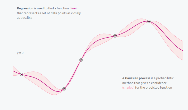参考：高斯过程直觉 此架构的概念基础。高斯过程是一种概率方法，它在预测函数周围生成一个置信区域（阴影带），而不仅仅是一条单线。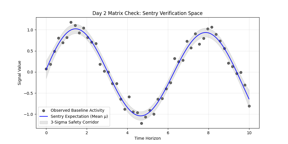  ### GP 后验拟合：合成验证 GP 从 60 个带噪声的锚点中正确学习到了一条平滑的潜在路径，并在 200 个预测位置对其进行了重构。灰色带为 3-sigma 安全走廊。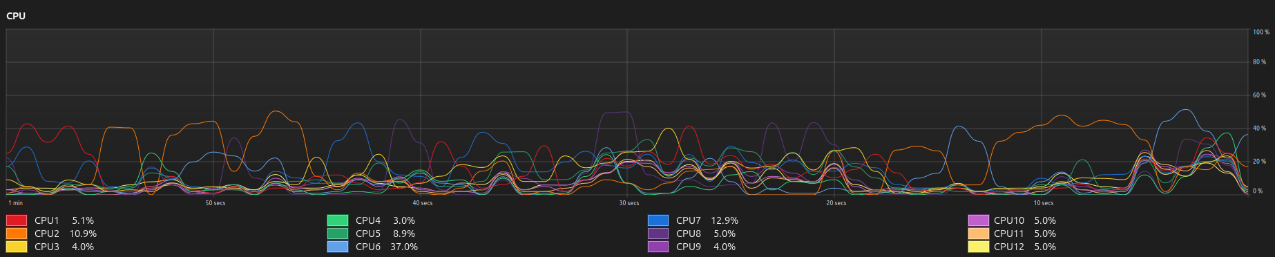  ### 系统监控器：硬件上下文 守护程序跟踪跨越所有 12 个核心的系统范围平均值。下方的逐核心视图展示了输入到复合 kernel 的原始利用率。  ## 数学基础 ### Kernel 任意两个时间点之间的协方差由径向基函数定义： $$k(x, x') = \sigma_f^2 \exp\left( -\frac{\|x - x'\|^2}{2l^2} \right)$$ - **Signal variance** 控制概率边界的垂直范围。 - **Length-scale** 控制模型的时间记忆，即过去多长时间内的数据点会影响当前预测。 ### 预测推理 给定一个新的时间点，引擎会计算： **预测均值：** $$\mu_* = K_*^\top [K + \sigma_n^2 I]^{-1} y$$ **预测方差：** ``` \sigma^2_{*} = K(X_{*}, X_{*}) - K_{*}^\top [K + \sigma_n^2 I]^{-1} K_{*} ``` 方差在靠近训练观测值的地方收缩，在未观测区域中扩大。3-sigma 走廊覆盖了 99.7% 的概率质量。 ## 阶段 1：合成信号验证 第一阶段针对带有高斯噪声的受控正弦波验证引擎。这确认了 GP 能够在引入任何实时数据之前正确重构潜在路径，并绘制出校准良好的置信走廊。 **信号生成器** (`utils/signal_gen.py`)： ``` import numpy as np def generate_signal(n_samples=60, noise_level=0.15): np.random.seed(42) X = np.linspace(0, 10, n_samples).reshape(-1, 1) y_clean = np.sin(X).ravel() noise = np.random.normal(0, noise_level, n_samples) return X, y_clean + noise ``` **哨兵引擎** (`core/sentry_engine.py`)： ``` from sklearn.gaussian_process import GaussianProcessRegressor from sklearn.gaussian_process.kernels import RBF, ConstantKernel as C class KernelSentry: def __init__(self, length_scale=1.0, noise_level=0.1): self.kernel = C(1.0, (1e-2, 1e2)) * RBF( length_scale=length_scale, length_scale_bounds=(1e-1, 1e2) ) self.gp = GaussianProcessRegressor( kernel=self.kernel, alpha=noise_level**2, n_restarts_optimizer=10, random_state=42 ) def learn(self, X, y): self.gp.fit(X, y) def check_integrity(self, X_new): return self.gp.predict(X_new, return_std=True) ``` ## 阶段 2：实时 CPU 遥测 第二阶段针对实时的 Linux 系统数据部署引擎。该模型以 CPU 利用率为目标，通过 `psutil` 每秒采样一次，并在 60 秒的滑动窗口上运行。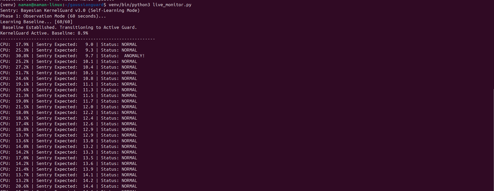 ### 复合 Kernel CPU 利用率包含三个结构组件，单一 RBF kernel 无法准确表示它们： | 组件 | Kernel | 用途 | |---|---|---| | 空闲基线偏移 | `ConstantKernel` | 处理非零基准（空闲机器上约为 6-12%） | | 应用负载趋势 | `RBF` | 随着进程的打开和关闭，对平滑的工作负载爬升进行建模 | | 中断抖动 | `WhiteKernel` | 吸收高频噪声，因此短暂的峰值不会被标记 | ### 自校准阶段 系统在激活异常检测之前，会运行一个强制性的 60 秒观测阶段。在此窗口期间，它会收集基线遥测数据并拟合初始模型。校准完成后，它将进入主动守护模式。 ### 实时监控器 (`live_monitor.py`)： ``` import psutil import numpy as np from sklearn.gaussian_process import GaussianProcessRegressor from sklearn.gaussian_process.kernels import RBF, WhiteKernel, ConstantKernel # 观察阶段 history_x = np.atleast_2d(np.linspace(0, 59, 60)).T history_y = [] while len(history_y) < 60: history_y.append(psutil.cpu_percent(interval=1)) history_y = np.array(history_y) initial_baseline = np.mean(history_y) kernel = ConstantKernel(constant_value=initial_baseline) \ + 1.0 * RBF(length_scale=10.0) \ + WhiteKernel(noise_level=1.0) gp = GaussianProcessRegressor(kernel=kernel) # 主动 guard loop while True: current_usage = psutil.cpu_percent(interval=1) history_y = np.roll(history_y, -1) history_y[-1] = current_usage gp.fit(history_x, history_y) mu, sigma = gp.predict(np.atleast_2d([60]).T, return_std=True) upper = mu[0] + 3 * sigma[0] lower = mu[0] - 3 * sigma[0] status = "ANOMALY" if current_usage > upper or current_usage < lower else "NORMAL" print(f"CPU: {current_usage:5.1f}% | Expected: {mu[0]:5.1f} | Status: {status}") ``` ### 观测到的行为 - 在校准期间学习到了 6.8% 的初始空闲基线。 - 当负载攀升至 13.4% 然后达到 19.6% 时，模型更新了其预期均值，并未触发误报；工作负载的偏移足够平缓，落在滑动窗口学习到的趋势范围内。 - 旨在标记违反概率安全走廊的突发非相关峰值。  ## 关键设计决策 **在线滑动窗口优于批量重新训练。** GP 每秒在固定的 60 个数据点窗口上重新拟合，而不是无限制地增加数据集。这保持了恒定的推理延迟，并确保模型跟踪当前行为而不是历史平均值。 **矩阵维度。** 所有时间数组在传递给 kernel 之前都被重塑为 `(-1, 1)`。线性代数后端在构建协方差矩阵时需要二维列矩阵。 **分辨率不对称。** 训练使用 60 个锚点。预测在 200 个位置运行。这产生了一个平滑、高分辨率的流形，而无需密集的训练数据。 **超参数优化。** RBF 的 length-scale 和 signal variance 通过在 `fit()` 期间最大化对数边际似然进行优化。初始 kernel 选择后无需手动调参。 ## 安装和使用 ``` # Clone the repository git clone https://github.com/thenamanshukla/gaussianguard.git cd gaussianguard # Create and activate virtual environment python -m venv venv source venv/bin/activate # Install dependencies pip install -r requirements.txt ``` **运行合成验证：** ``` python examples/detector_demo.py ``` 输出：`gp_verification.png` — 针对带噪声正弦信号的后验拟合图。 **运行实时 CPU 守护程序：** ``` python live_monitor.py ``` 终端将显示 60 秒的校准进度，然后切换到实时异常报告。 ## 依赖要求 ``` numpy scikit-learn matplotlib psutil ``` ## 参考文献 Rasmussen, C. E., and Williams, C. K. I. *Gaussian Processes for Machine Learning*. MIT Press, 2006. Distill.pub. *A Visual Exploration of Gaussian Processes*. 2019. https://distill.pub/2019/visual-exploration-gaussian-processes/

标签：Apex, 异常检测, 时间序列分析, 机器学习, 贝叶斯推断, 逆向工具, 高斯过程回归