MetrPikeska/roundabout-exit-detection

# 环形交叉路口交通分析 – 基于视觉的 GIS 流水线 使用 YOLOv8 + ByteTrack 结合地理参考单应性标定，对环形交叉路口的车辆和行人进行自动检测、跟踪和空间分析。输出包括 GeoPackage/GeoTIFF 图层，可直接导入 QGIS 或 PostGIS。 ## 结果 处理了**5分钟**的航拍镜头（Kopřivnice，Obránců míru 交叉路口）： | 指标 | 值 | |---|---| | 检测到的车辆（轨迹 ≥ 5 个点） | **142**（130辆乘用车，12辆卡车） | | 平均运行速度 | **23.1 km/h** | | 第85百分位速度 | **31.9 km/h** | | 平均轨迹长度 | **46.6 m** | | 记录的驶离交叉总次数 | 5分钟内 **93** 次 | | 高峰流量 | **23 辆/分钟**（第4分钟） | | 主要 O/D 流向 | SW（西南）入口 → NE（东北）入口（25辆车，26 %） | | 出口加速度（驶离阶段） | **29.8 km/h**，而驶近时为 20.8 km/h | | 检测到的车辆-行人冲突 | **139**（132次 SW 横穿，7次 NE 横穿） | **单应性标定：** 来自 ČÚZK 正射影像的 11 个地面控制点（QGIS，S-JTSK EPSG:5514）。 平均重投影误差：**0.51 m**，最大 **0.97 m**。 速度估计未与 GPS 参考进行验证。对 3 个经过的样本进行人工比对：误差在约 ±3 km/h 范围内一致。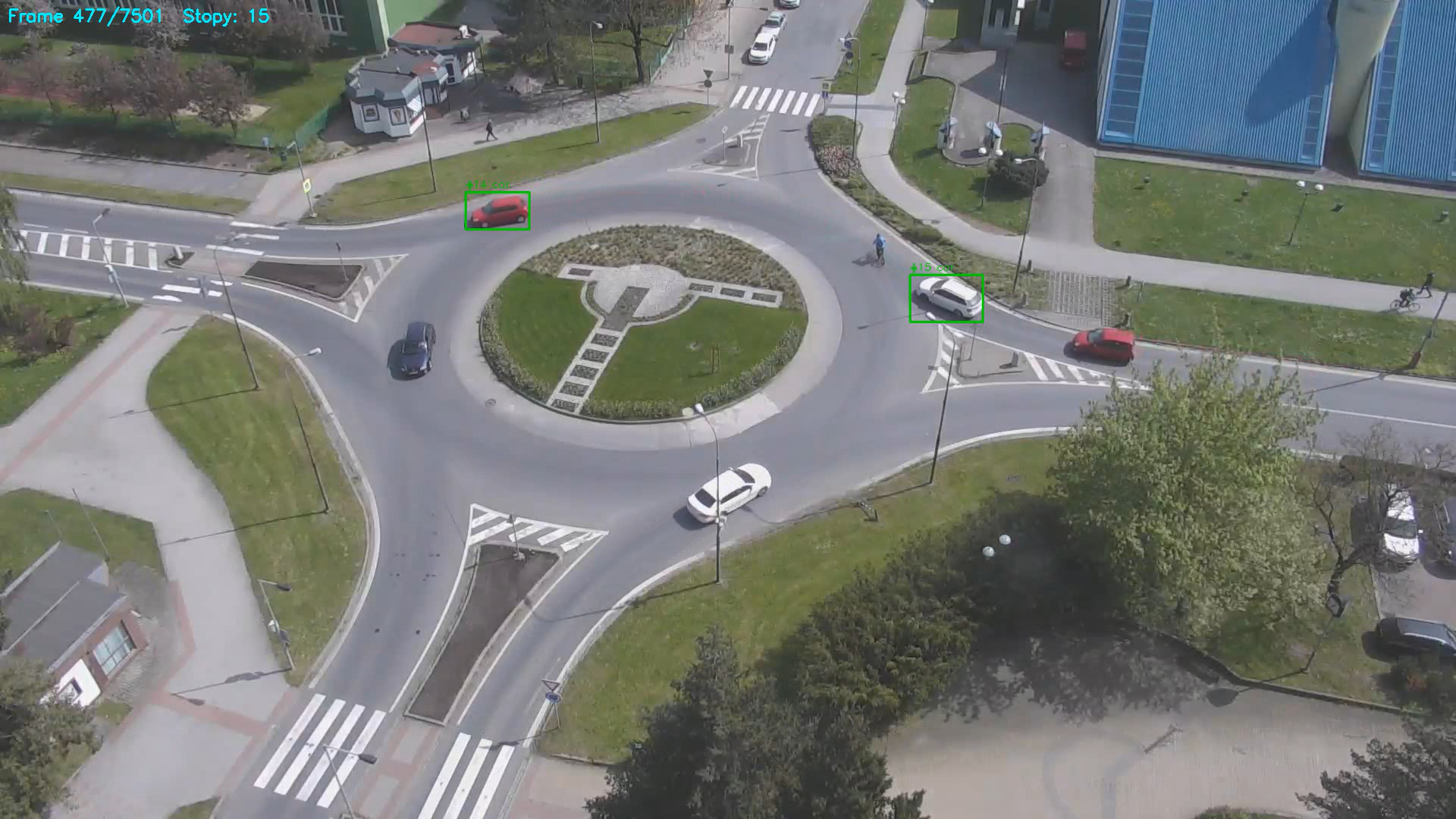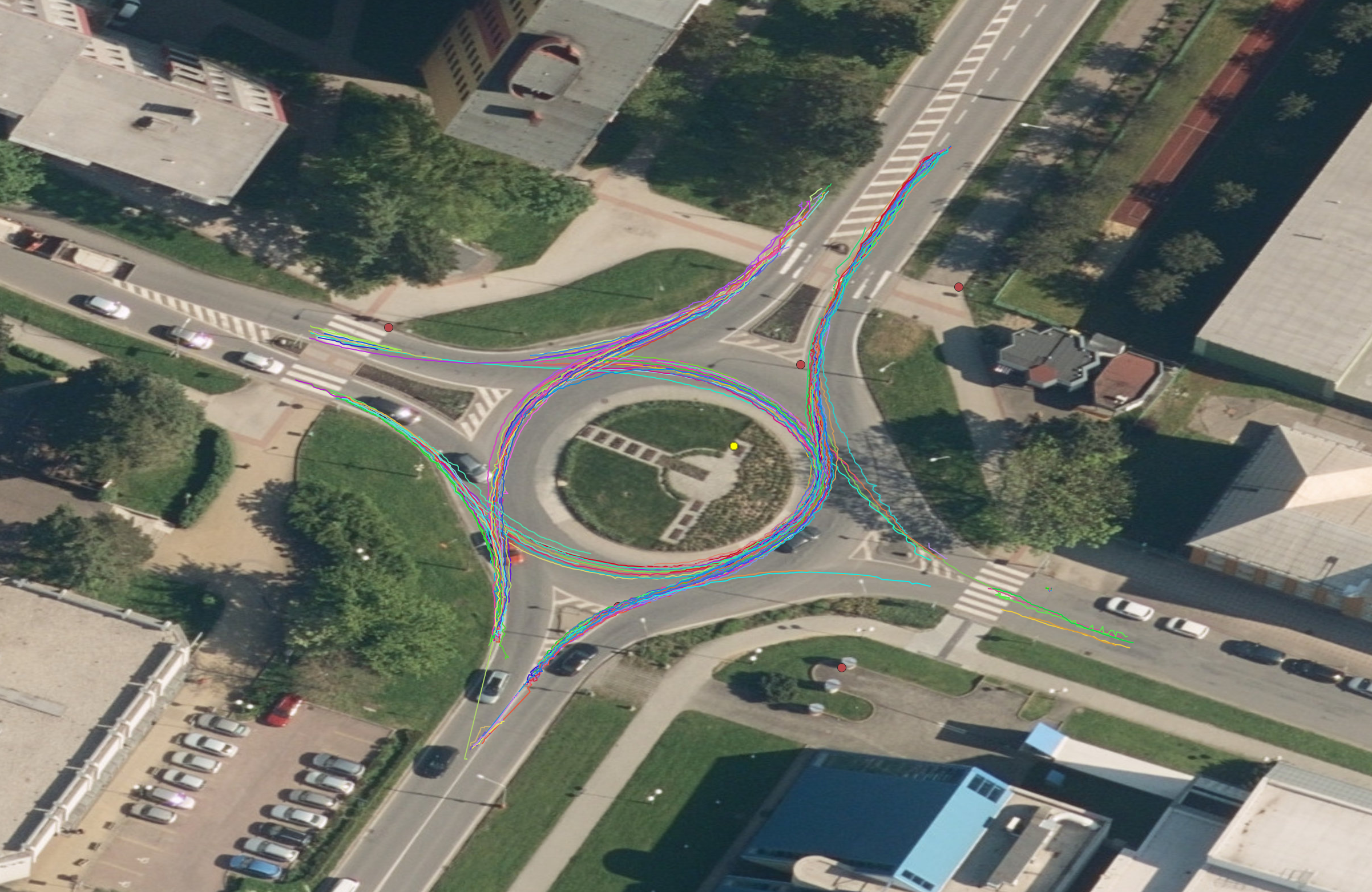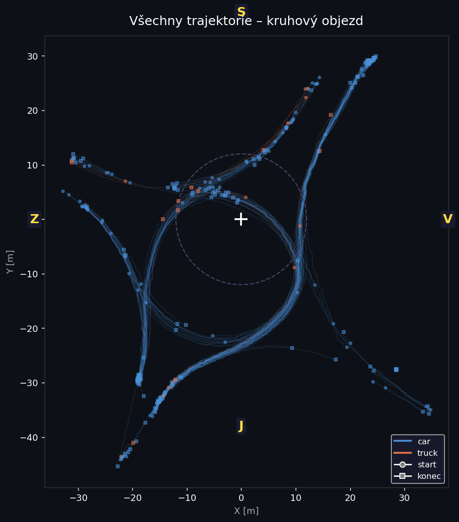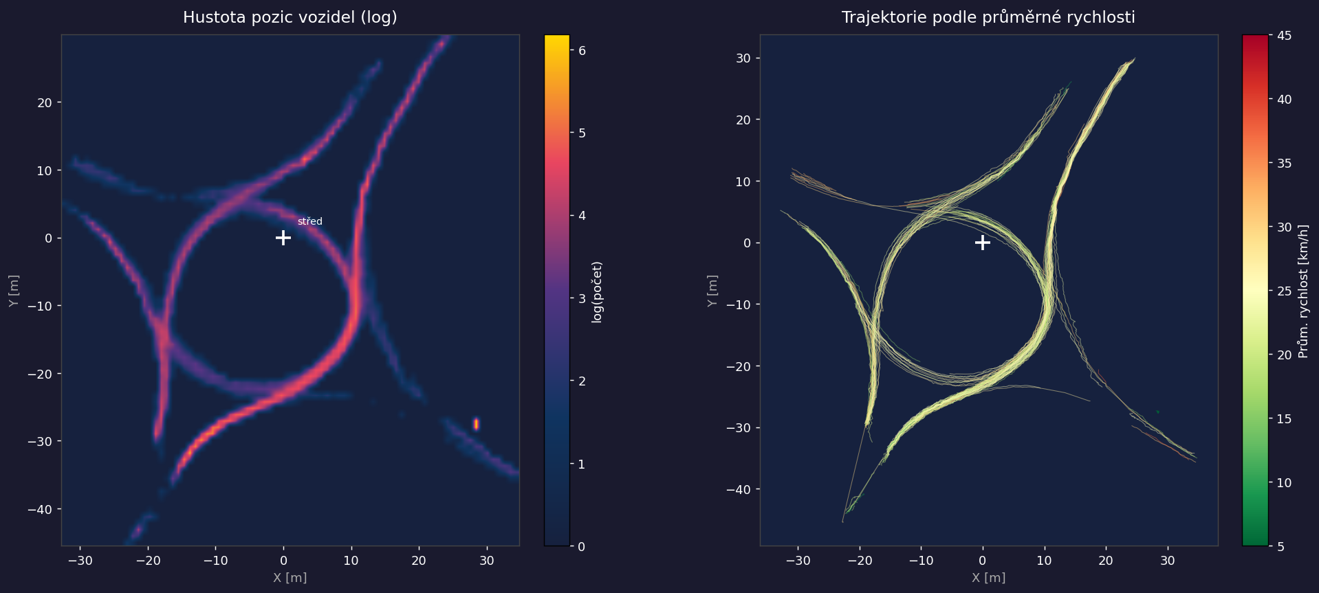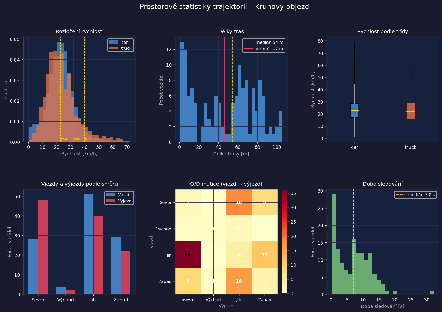 ## 输出示例 **车辆跟踪回放（YOLOv8 + ByteTrack，带有瞬时速度的轨迹拖尾）：**  **检测输出帧：**  **GIS 可视化 – 正射影像上的轨迹（QGIS）：**  ## 空间统计 `spatial_stats.py` 读取 `data/tracks.pkl` 并在 `output/` 中生成三种可视化图表。 ``` python spatial_stats.py ```    ## 项目结构 该项目为不同的分析目标提供了**两个独立的工作流**： ``` roundabout-exit-detection/ │ │ ── Workflow A: Exit counting (pixel-space) ────────────────── ├── define_exclusion.py # interactive exclusion zone definition ├── 01_detect_and_count.py # YOLOv8 + pixel polygons → CSV │ └── output/car_crossings.csv (flow per exit per minute) │ │ ── Workflow B: GIS tracking pipeline ──────────────────────── ├── extract_frame.py # frame extraction for calibration ├── calibrate.py # GCP clicking → homography.npy ├── detect_track.py # YOLOv8 + ByteTrack + homography → pkl ├── speed_estimator.py # speed computation module (importable) ├── export_geo.py # tracks.pkl → GeoPackage (QGIS/PostGIS) │ │ ── Analysis modules ───────────────────────────────────────── ├── spatial_stats.py # spatial statistics + visualisations │ └── output/stats_*.png ├── od_matrix.py # origin–destination matrix between arms │ └── output/od_matrix.csv ├── speed_profile.py # speed profile per phase (approach/circulating/departure) │ └── output/speed_profile.csv + speed_profile.png ├── heatmap.py # movement density → GeoTIFF + PNG preview │ └── output/heatmap.tif (EPSG:4326) + heatmap_preview.png ├── pedestrian_conflicts.py # vehicle × pedestrian conflicts at crossings │ └── output/conflicts.csv ├── export_postgis.py # export tracks + conflicts → PostGIS schema │ ├── data/ │ ├── frames/ # extracted calibration frames │ ├── gcp/ # GCP shapefile (EPSG:4326, 11 points) │ ├── gcps.csv # GCP table (pixel + world coordinates) │ ├── homography.npy # 3×3 homography matrix (gitignored) │ ├── tracks.pkl # track history {id: [(x, y, frame)]} (gitignored) │ └── tracks.gpkg # GeoPackage: tracks + positions layers (gitignored) ├── output/ │ ├── car_crossings.csv │ ├── od_matrix.csv │ ├── speed_profile.csv + .png │ ├── heatmap.tif + heatmap_preview.png │ ├── conflicts.csv │ └── stats_*.png └── requirements.txt ``` ## 安装说明 ``` python -m venv .venv source .venv/bin/activate # Linux / macOS # .venv\Scripts\Activate.ps1 # Windows PowerShell pip install -r requirements.txt ``` **GPU（推荐）：** ``` pip install torch torchvision torchaudio --index-url https://download.pytorch.org/whl/cu121 pip install -r requirements.txt ``` ## 流水线 ### 步骤 1 – 帧提取 ``` python extract_frame.py "data/recording.avi" ``` 保存 `data/frames/frame_0000s.png`、`frame_0060s.png`、… 并将第 0 帧复制为 `frame_ref.png` 用于标定。 ### 步骤 2 – 地面控制点 填充 `data/gcps.csv`。列 `world_x_m` 和 `world_y_m` 是相对于交叉路口中心的以米为单位的坐标： ``` id,description,pixel_x,pixel_y,world_x_m,world_y_m,lon_wgs84,lat_wgs84 1,ne_entry_kerb,,,−12.5,38.2,, 2,se_lane_marking,,,42.1,5.0,, ``` 有关从 QGIS 获取坐标的信息，请参见**第 4 节**。 ### 步骤 3 – 单应性标定 ``` python calibrate.py ``` 显示参考帧并提示按顺序点击 GCP。确认后保存： - `data/homography.npy` – 单应性矩阵 - 像素坐标回写到 `data/gcps.csv` 目标重投影误差：平均值 < 0.5 m。数值高于 2 m 表示存在问题。 ### 步骤 4 – 检测与跟踪 ``` python detect_track.py python detect_track.py --model yolov8s.pt --conf 0.30 --device 0 ``` 输出： - `data/tracks.pkl` – 世界坐标系下的轨迹历史 - `data/tracks_annotated.mp4` – 标注后的视频 ### 步骤 5 – GIS 导出 编辑 `export_geo.py`：将 `REF_X_SJTSK` 和 `REF_Y_SJTSK` 设置为交叉路口中心的实际 S-JTSK 坐标（见第 4 节）。 ``` python export_geo.py ``` `data/tracks.gpkg` 包含两个图层： - **tracks** – 每辆车一条 LineString（速度、类别、时间戳） - **positions** – 每次检测为一个 Point ### 步骤 6 – 分析模块 独立运行任何模块： ``` python od_matrix.py # origin–destination matrix python speed_profile.py # speed by phase python heatmap.py # movement density GeoTIFF python pedestrian_conflicts.py # vehicle × pedestrian conflicts (full video) python spatial_stats.py # combined visualisations ``` ### 步骤 7 – PostGIS 导出 ``` python export_postgis.py --db gis --user postgres --drop ``` 在 EPSG:4326 中创建带有空间索引的 `roundabout` 模式以及 `tracks`、`positions`、`conflicts` 表。有关连接选项，请参见 `export_postgis.py --help`。 ## 从 QGIS 获取 GCP 坐标 ### QGIS（推荐 – 亚米级精度） 1. 打开 QGIS → 项目 → 属性 → CRS → 设置为 **EPSG:5514**（S-JTSK/Krovak East North） 2. 添加正射影像底图（WMS/WMTS）： - ČÚZK 正射影像：`https://ags.cuzk.cz/arcgis1/services/ORTOFOTO/MapServer/WMSServer` 3. 导航至交叉路口 4. 从状态栏读取交叉路口中心坐标 → 这些即为 `REF_X_SJTSK`、`REF_Y_SJTSK` 5. 对于每个 GCP，在帧图像上点击并计算： - `world_x_m = gcp_easting − REF_X_SJTSK` - `world_y_m = gcp_northing − REF_Y_SJTSK` ### 坐标转换（Python） ``` from pyproj import Transformer t = Transformer.from_crs("EPSG:4326", "EPSG:5514", always_xy=True) x_sjtsk, y_sjtsk = t.transform(lon, lat) ``` ## 在 QGIS 中打开 tracks.gpkg 1. **图层 → 添加图层 → 添加矢量图层** → 选择 `data/tracks.gpkg` 2. 添加两个图层（tracks + positions） 3. 将项目 CRS 设置为 **EPSG:4326** 或 **EPSG:5514** 4. 要可视化速度：右键点击 tracks 图层 → 属性 → 符号化 → 渐变 → 字段 `speed_avg_kmh` ## 注意事项 - 单应性精度仅限于道路表面平面。在具有强烈透视畸变的帧边缘附近的车辆，其位置精度可能会降低。 - `speed_estimator.py` 会过滤掉低于 1 km/h（静止车辆）和高于 80 km/h（错误检测）的速度。 - FPS 通过 `cap.get(cv2.CAP_PROP_FPS)` 从视频中自动读取。 - `yolov8n.pt` 在首次运行时自动下载（约 6 MB）。`yolov8s.pt`（约 22 MB）提供更高的检测精度。

标签：ByteTrack, GeoJSON, GeoPackage, GeoTIFF, GIS, PostGIS, QGIS, Shapely, YOLOv8, 交通流量分析, 冲突检测, 凭据扫描, 单应性矩阵, 地理配准, 多边形ROI, 数据导出CSV, 智能交通系统, 热力图, 状态机, 环形交叉路口, 目标检测, 空间分析, 行人检测, 计算机视觉, 车辆追踪, 轨迹分析, 逆向工具, 速度估算